Logistic Regression and the S&P 500

Today I learned about Logistic Regression and applied it to the S&P500 to predict tomorrow’s movement, up or down. Something that can be used for prediction markets.

Linear Regression attempts to quantify a specific value, like predicting the exact value of a stock each day.

Logistic Regression is a classification algorithm. It doesn’t care about exact numbers, only movement, up or down.

With a Bachelor in Finance, I was quite surprised to not have been exposed to this model. Very interesting and quite useful.

For this project, I used 5 years of data of SPY to train the model. I imported the necessary libraries and downloaded the data with yfinance.

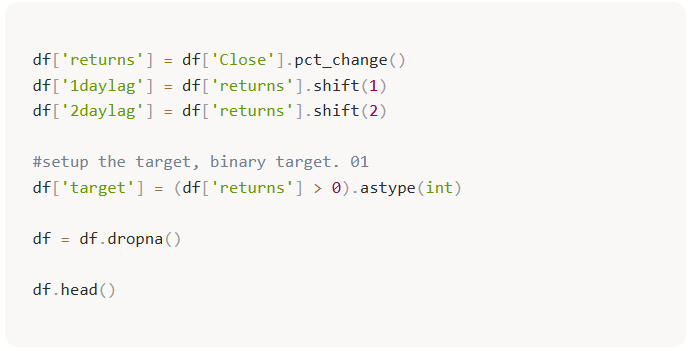
Afterwards, we needed to manipulate the dataframe a bit. We need our model inputs. For this project I decided to keep it simple and only included 2 lags: 1 day returns and 2 day returns.

The preprocessing steps

Calculate Returns: we transform raw prices into daily percentage changes.
Create Lags: we use shift(1) and shift(2) to create features based on the previous two days.
Define the Target: we use astype(int) to create a binary target: 1 if the price went up, and 0 if it stayed flat or dropped.
Lookahead Bias: by using lags as features (X), we ensure the model only sees what happened yesterday to predict tomorrow. If the model sees today’s data to predict today’s price, it’s not learning, it’s cheating.

Code snippet defining returns, lagged features, and the binary target for the logistic regression model.

Afterwards, we need to separate the data between training and testing. A split of 80/20 is perfect for these models, but there is no defined combination. Normally, it is ideal to keep the training data ratio higher than the testing. The more the model can learn, the more accurate it can be.

Code snippet splitting the dataset into training and testing sets using an 80/20 ratio.

We are now ready to train the model. Using the sklearn library we initially imported, we use .fit() to train the model.

Code snippet fitting the logistic regression model using the training data.

Here I learned about the C parameter in the model. Regularization. It is essentially the level of strictness of the model. I kept the C relatively high for this project, so overfitting might be present.

Table explaining underfitting, optimal fit, and overfitting, and how changing the C parameter affects each case.

Illustration comparing underfitting, optimal fit, and overfitting decision boundaries.

In the next step we used the model on our test data. The results were as expected.

Code snippet showing the model predictions, confusion matrix, and accuracy values on the test data.

Looking at the summary statistics of the model, we can see that neither of the indicators is significantly relevant at predicting the next day’s price. It proves the model was guessing and relying on the overall trend of the market. A p-value of 0.3 is basically noise.

Logit regression results table showing coefficients and p-values for the lag variables.

Flaws and biases

The model predicted the market would go “Up” 261 times out of 263.
The problem: it only predicted “Down” 2 times.
The bullish trap: because the S&P 500 tends to go up over time, the model learned that by simply saying “Up” constantly, it can maintain a 57% accuracy rate without actually understanding the market’s randomness.
The 70% confidence threshold: when I raised the requirement to a 70% probability, the accuracy plummeted to 42.5%. This is the most honest part of the results. It shows that when the model is “sure” of itself, it is actually less accurate than a random guess. In prediction markets, this becomes a signal in reverse. You would almost be better off doing the opposite of what the model suggests when its confidence is high.

Code snippet showing the predicted probability of the S and P 500 going down or up tomorrow.

Conclusion

A good lesson between accuracy and truth. While the model had an accuracy above 50%, the confusion matrix revealed a strong bullish bias. The model didn’t find a pattern, it just found a trend.

In the future, looking beyond price lags and including signals such as Volatility, Moving Averages, and Volume can probably increase the model accuracy.

This was the first of many projects coming on the way. I am not chasing fame. I want a diary of my own for learning and maybe inspire others to do the same. I don’t call myself a quant or want to be one. Each failed model is just another iteration.

Enjoy the walk.